How To Solve Least Square Method. Form the augmented matrix for the matrix equation a t ax = a t b , and row reduce. The method of least squares is a procedure to determine the best fit line to data;

Note that we expect α 1 = 1.5 and α 2 = 1.0 based on this data. Form the augmented matrix for the matrix equation a t ax = a t b , and row reduce. It gives the trend line of best fit to a time series data.

How To Solve The Damped Wave Equation. With initial conditions u(x,0)=f(x), u t (x,0)=g(x) and boundary conditions u(0,t)=0 and u x (l,t)=0. In this work, the damped vibration of a string with fixed ends is considered.

If your sine curve is exponentially damped, drawing a line from peak to peak will result in an exponential decay curve, which has the general formula n(t) = a e (kt). You can edit the initial values of both u and u t by clicking your mouse on the white frames on the left. We make a complete deduction of its fundamental solutions, both for positive and negative times.

How To Solve A Second Order Differential Equation In Matlab. Using matlab to solve differential equations this tutorial describes the use of matlab to solve differential equations. An example is displayed in figure 3.3.

Differentiate your equation to get rid of it. For example one of the systems has the following set of 3 second order ordinary differential equations: The dsolve function finds a value of c1 that satisfies the condition.

How To Solve First Order Pde. We begin by nding the characteristic curve. A(x,y,u) ∂u ∂x +b(x,y,u) ∂u ∂y = c(x,y,u).

Pde=d [u [x,t],t]+d [u [x,t],x]==0; X =ξ, s =0 on t =0. Our notation lets z(s) =u(x(s)) and p i(s) =u xi (x(s)), so we consider f(p;z;x).

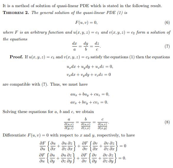
How To Solve Quasi Linear Pde. In general any linear combination of solutions c 1u 1(x;y) + c 2u 2(x;y) + + c nu n(x;y) = xn i=1 c iu i(x;y) will also solve the equation. Methods of solving partial differential equations 9.

2 solution define a curve in the x,y,u space as follows Numerical methods for solving pdes numerical methods for solving different types of pde's reflect the different character of the problems. Theorem the general solution to the transport equation ∂u ∂t +v ∂u ∂x = 0 is given by u(x,t) = f(x −vt), where f is any differentiable function of one variable.